The R package visStatistics allows for rapid
visualisation and statistical analysis of raw data. It
automatically selects and visualises the most appropriate
statistical hypothesis test between two vectors of
class integer, numeric or
factor.
This workflow is particularly suited for browser-based interfaces that rely on server-side R applications connected to secure databases, where users have no direct access, or for quick data visualisation, e.g. in statistical consulting projects.
install.packages("visStatistics")library(visStatistics)devtools from CRAN if not already installed:install.packages("devtools")devtools
package:library(devtools)visStatistics package from GitHub:install_github("shhschilling/visStatistics")visStatistics package:library(visStatistics)? visstatThe function visstat() accepts input in two ways:
# Standardised form (recommended):
visstat(x, y)

# Backward-compatible form:
visstat(dataframe, "name_of_y", "name_of_x")
In the standardised form, x and y must be
vectors of class "numeric", "integer", or
"factor".
In the backward-compatible form, "name_of_x" and
"name_of_y" must be character strings naming columns in a
data.frame named dataframe. These column must
be of class "numeric", "integer", or
"factor". This is equivalent to writing:
visstat(dataframe[["name_of_x"]], dataframe[["name_of_y"]])To simplify the notation, throughout the remainder, data of class
numeric or integer are both referred to by
their common mode numeric,
while data of class factor are referred to as
categorical.
The interpretation of x and y depends on
their classes:
If one is numeric and the other is a factor, the numeric must be
passed as response y and the factor as predictor
x. This supports tests for central tendencies.
If both are numeric, a simple linear regression model is fitted
with y as the response and x as the
predictor.
If both are factors, a test of association is performed
(Chi-squared or Fisher’s exact). The test is symmetric, but the plot
layout depends on which variable is supplied as x.
visstat() selects the appropriate statistical test and
generates visualisations accompanied by the main test statistics.
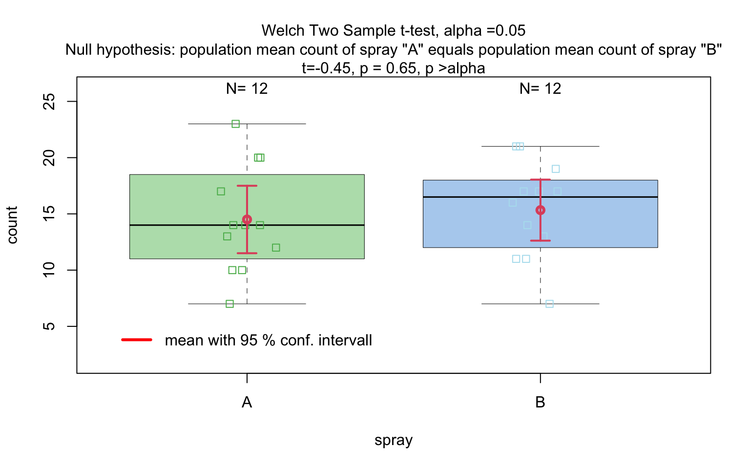
library(visStatistics)When the response is numerical and the predictor is categorical, test of central tendencies are selected.
insect_sprays_ab <- InsectSprays[InsectSprays$spray %in% c("A", "B"), ]
insect_sprays_ab$spray <- factor(insect_sprays_ab$spray)

# Standardised
visstat(insect_sprays_ab$spray, insect_sprays_ab$count)
# Backward-compatible function call resulting in same output
# visstat(insect_sprays_ab,"count", "spray")mtcars$am <- as.factor(mtcars$am)
t_test_statistics <- visstat(mtcars$am, mtcars$mpg)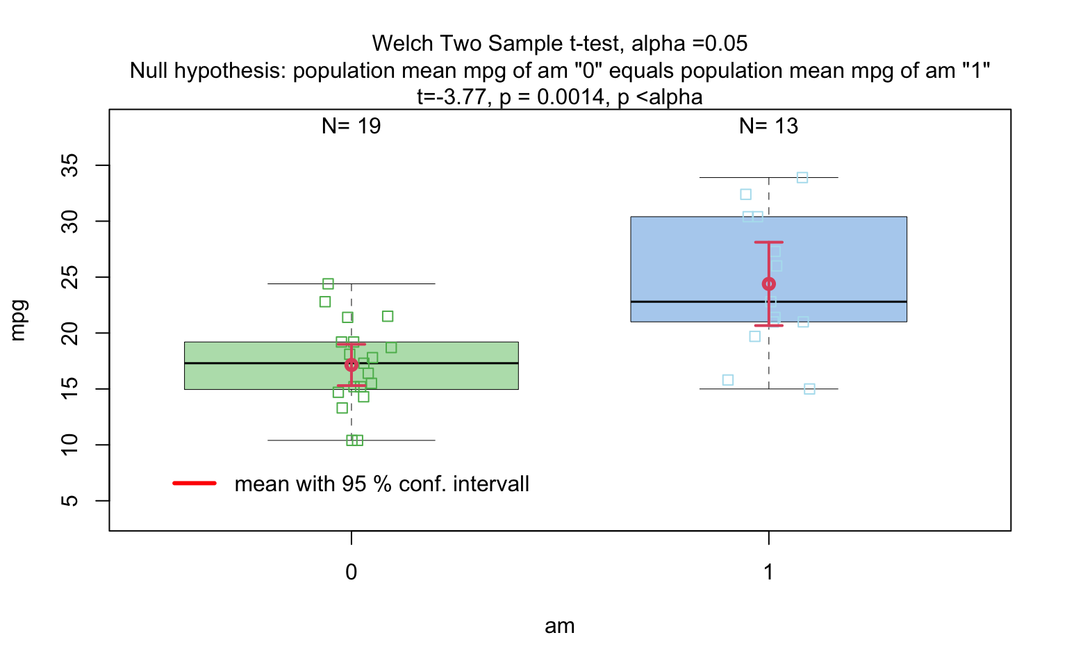
# t_test_statisticsgrades_gender <- data.frame(
sex = factor(rep(c("girl", "boy"), times = c(21, 23))),
grade = c(
19.3, 18.1, 15.2, 18.3, 7.9, 6.2, 19.4, 20.3, 9.3, 11.3,
18.2, 17.5, 10.2, 20.1, 13.3, 17.2, 15.1, 16.2, 17.0, 16.5, 5.1,
15.3, 17.1, 14.8, 15.4, 14.4, 7.5, 15.5, 6.0, 17.4, 7.3, 14.3,
13.5, 8.0, 19.5, 13.4, 17.9, 17.7, 16.4, 15.6, 17.3, 19.9, 4.4, 2.1
)
)
wilcoxon_statistics <- visstat(grades_gender$sex, grades_gender$grade)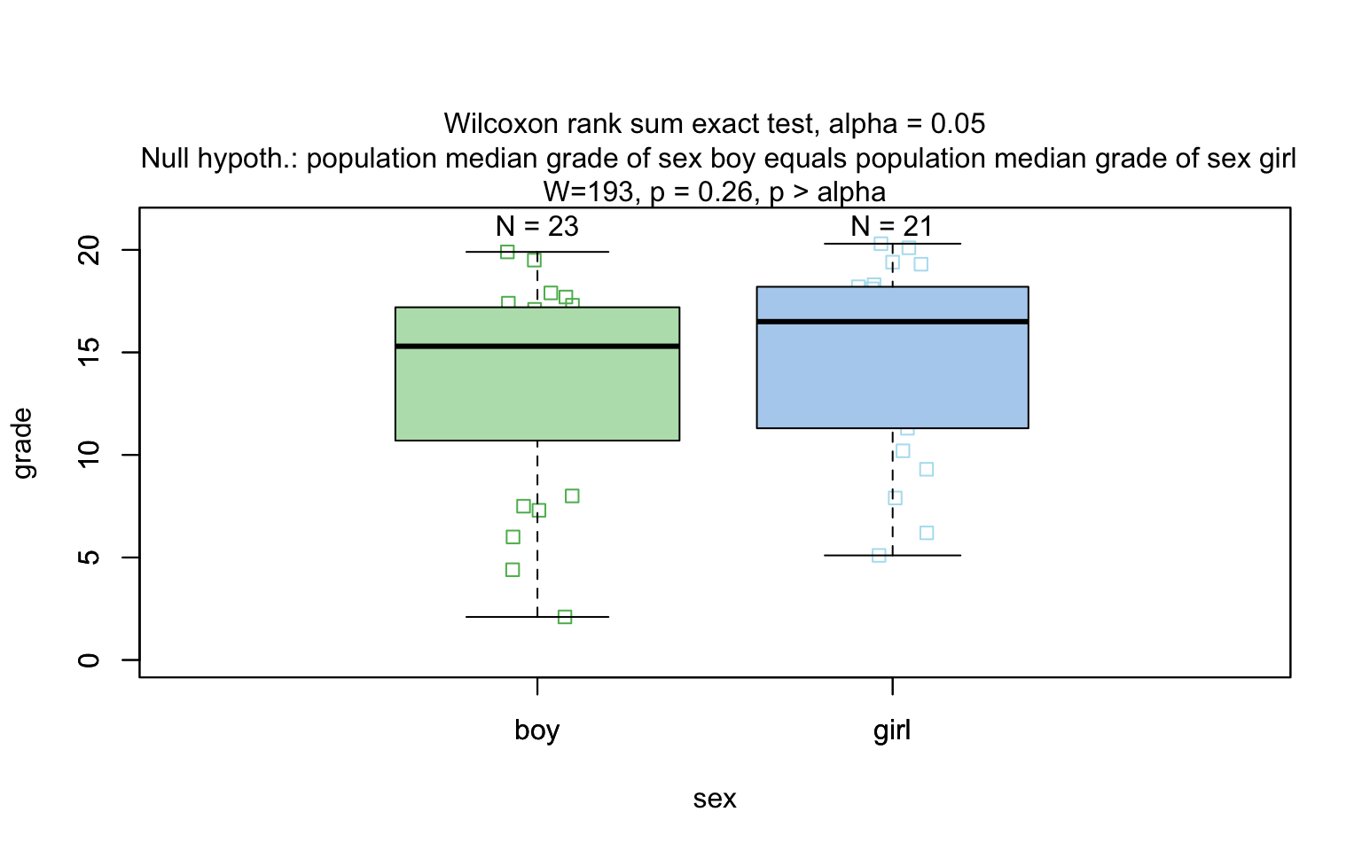
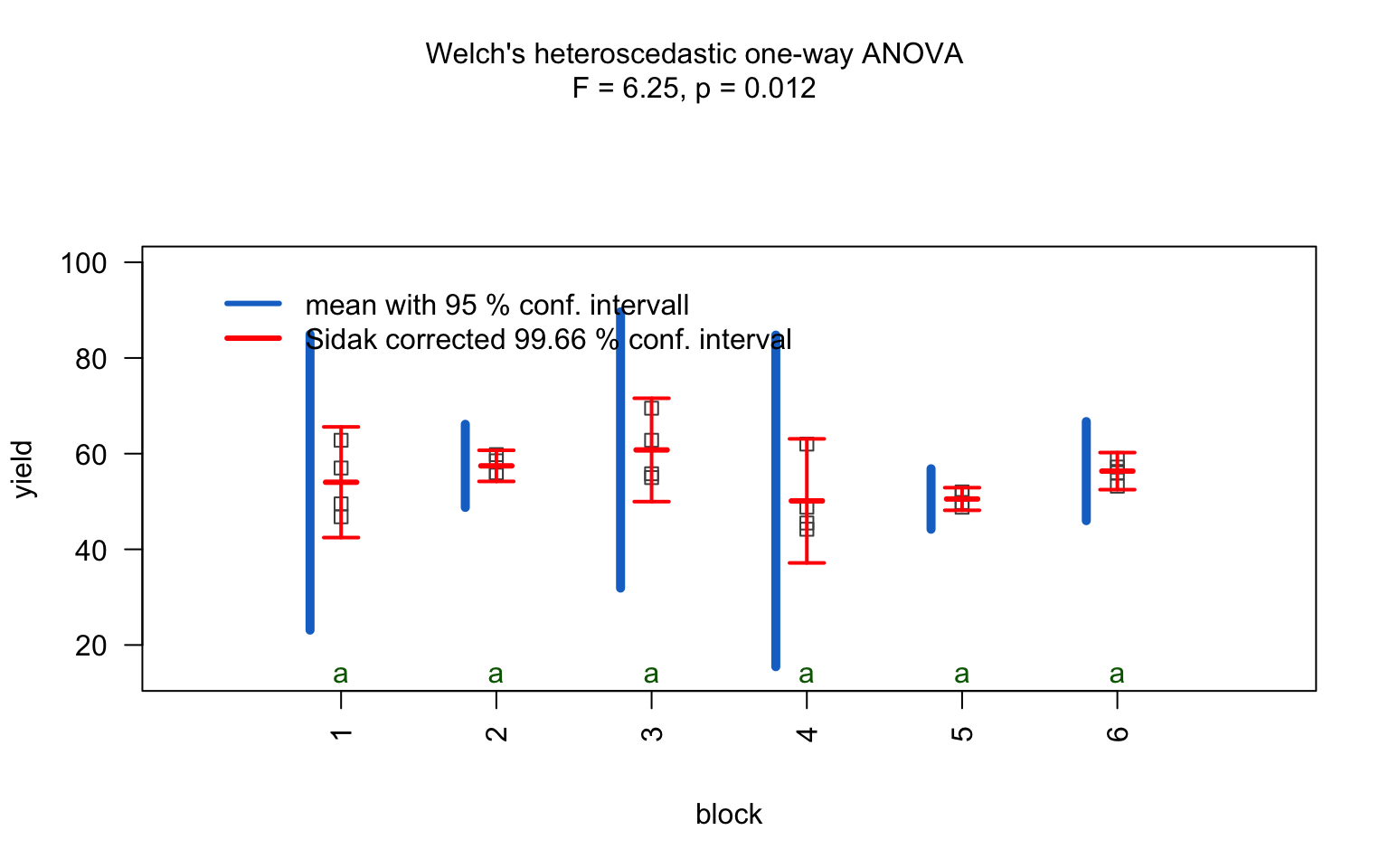
one_way_npk <- visstat(npk$block,npk$yield)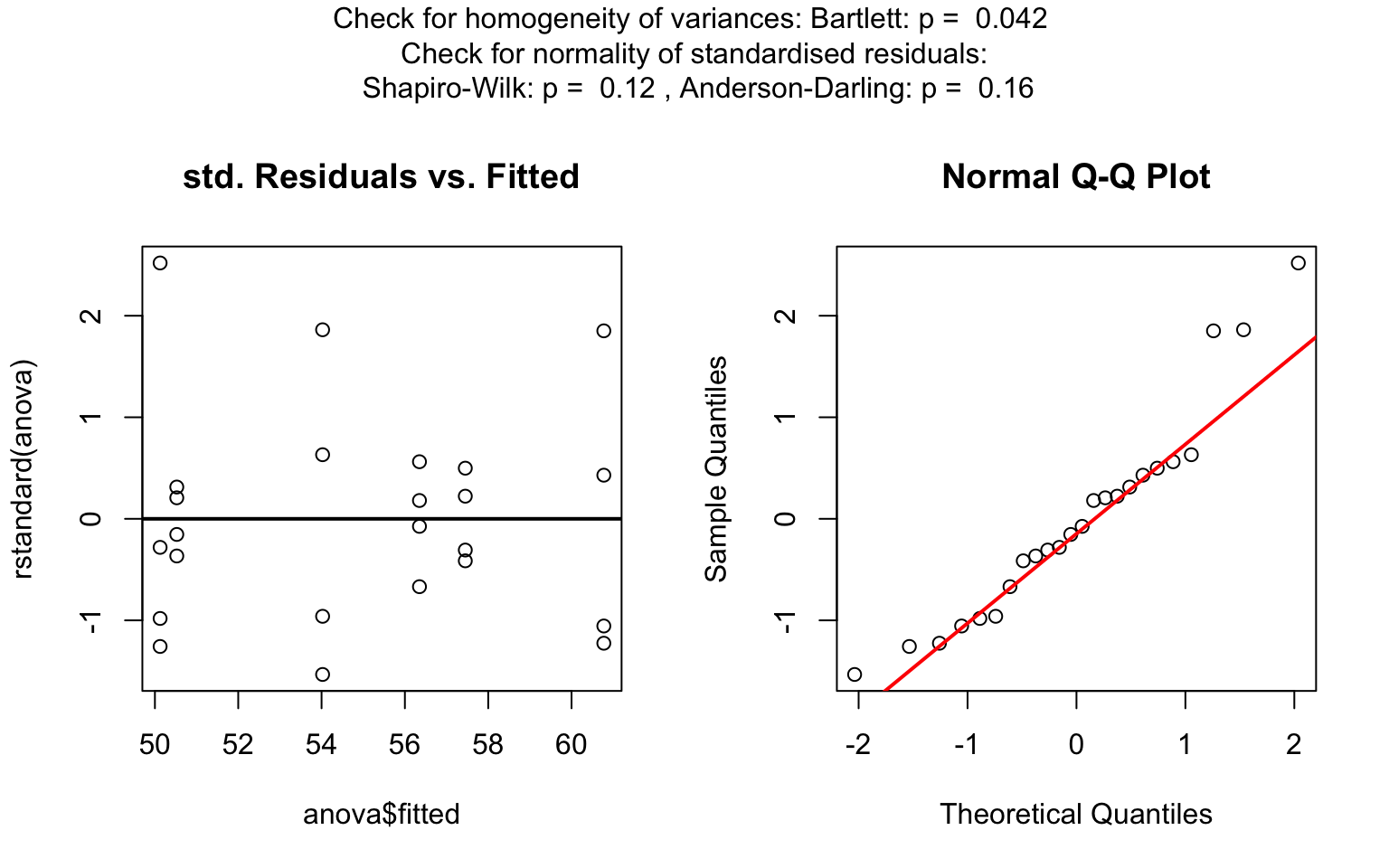
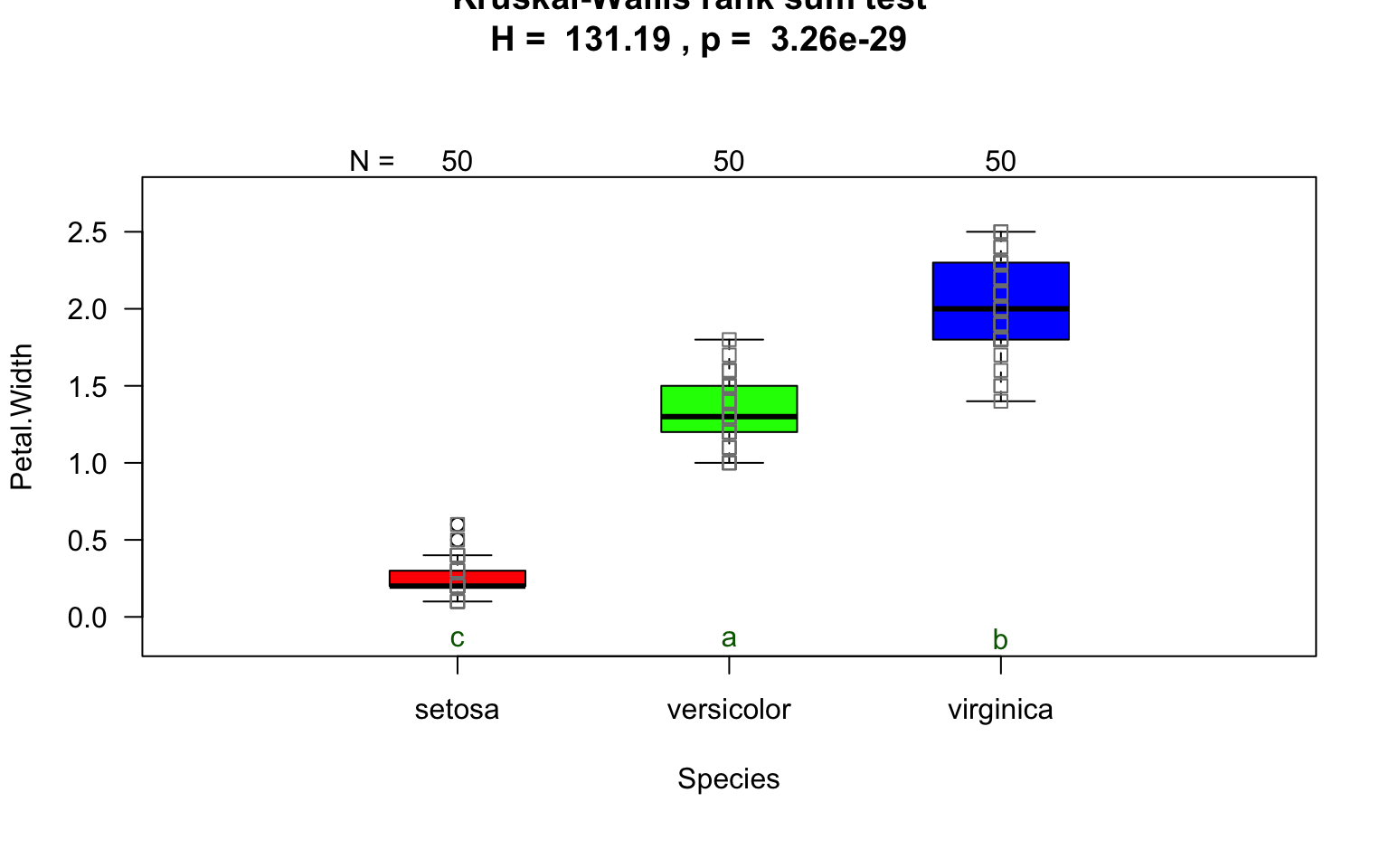
visstat(iris$Species, iris$Petal.Width)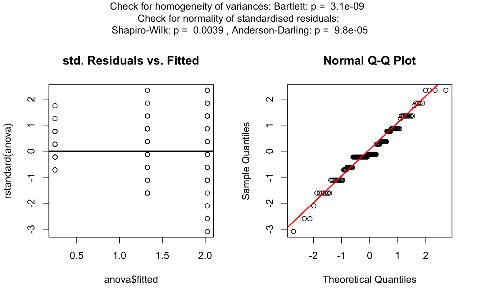
 The generated graphs can be saved in all available formats of the
Cairo package. Here we save the graphical output of type
“pdf” in the plotDirectory tempdir():
visstat(
iris$Species,iris$Petal.Width,graphicsoutput = "pdf",plotDirectory = tempdir()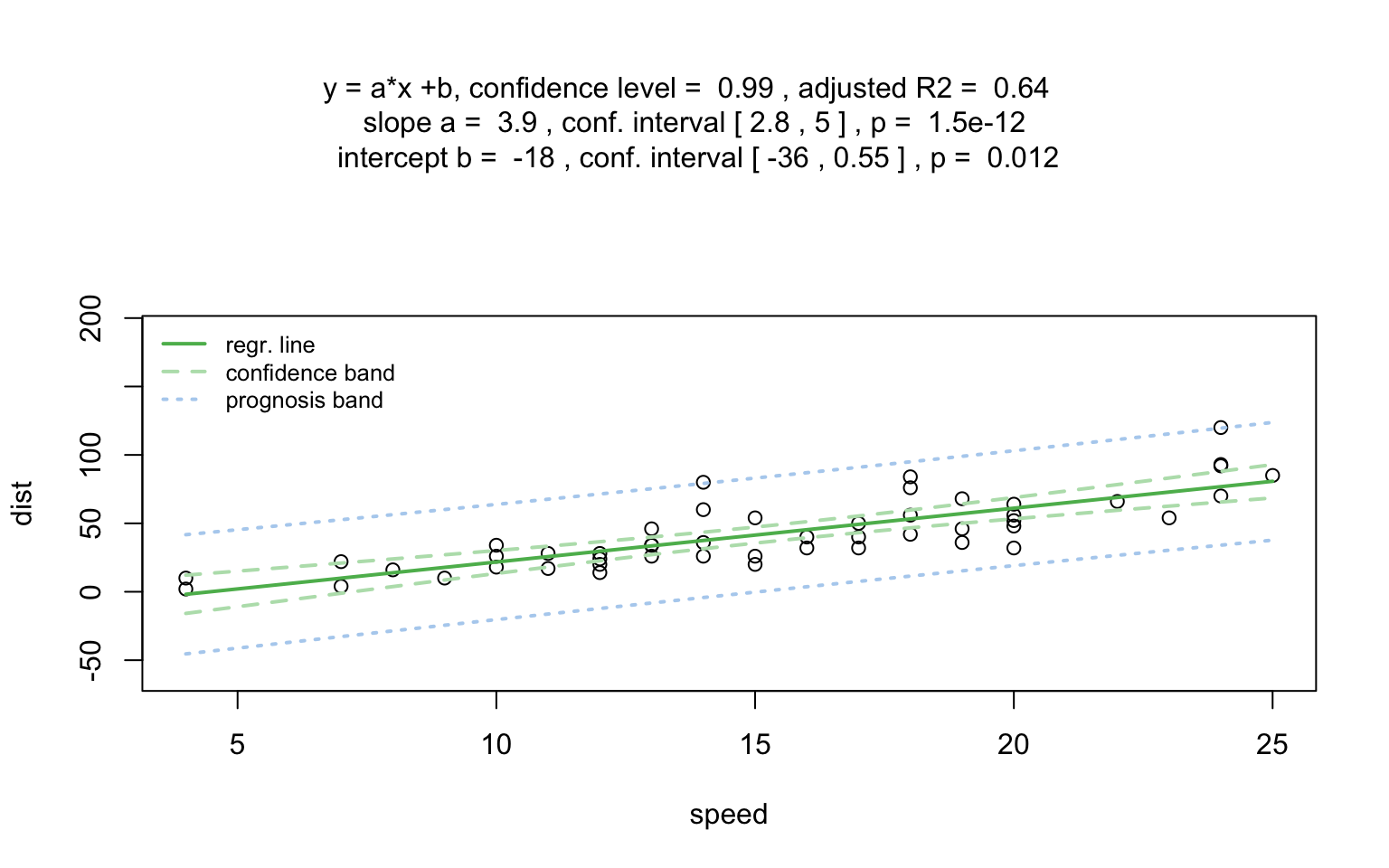
)linreg_cars <- visstat(cars$speed ,cars$dist)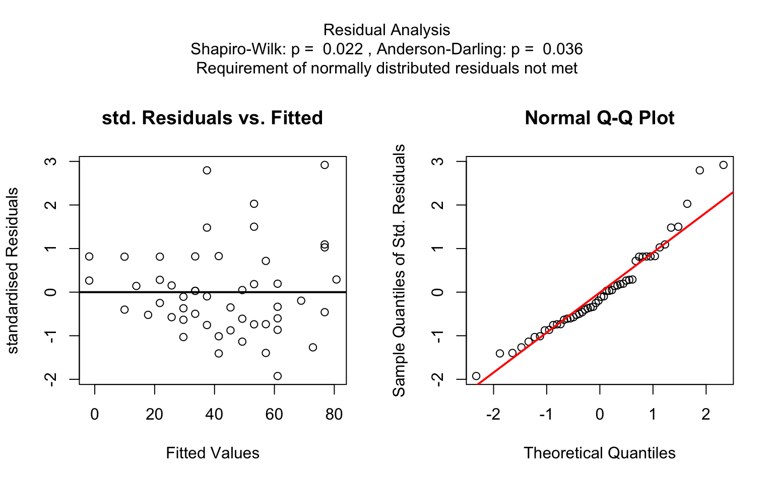
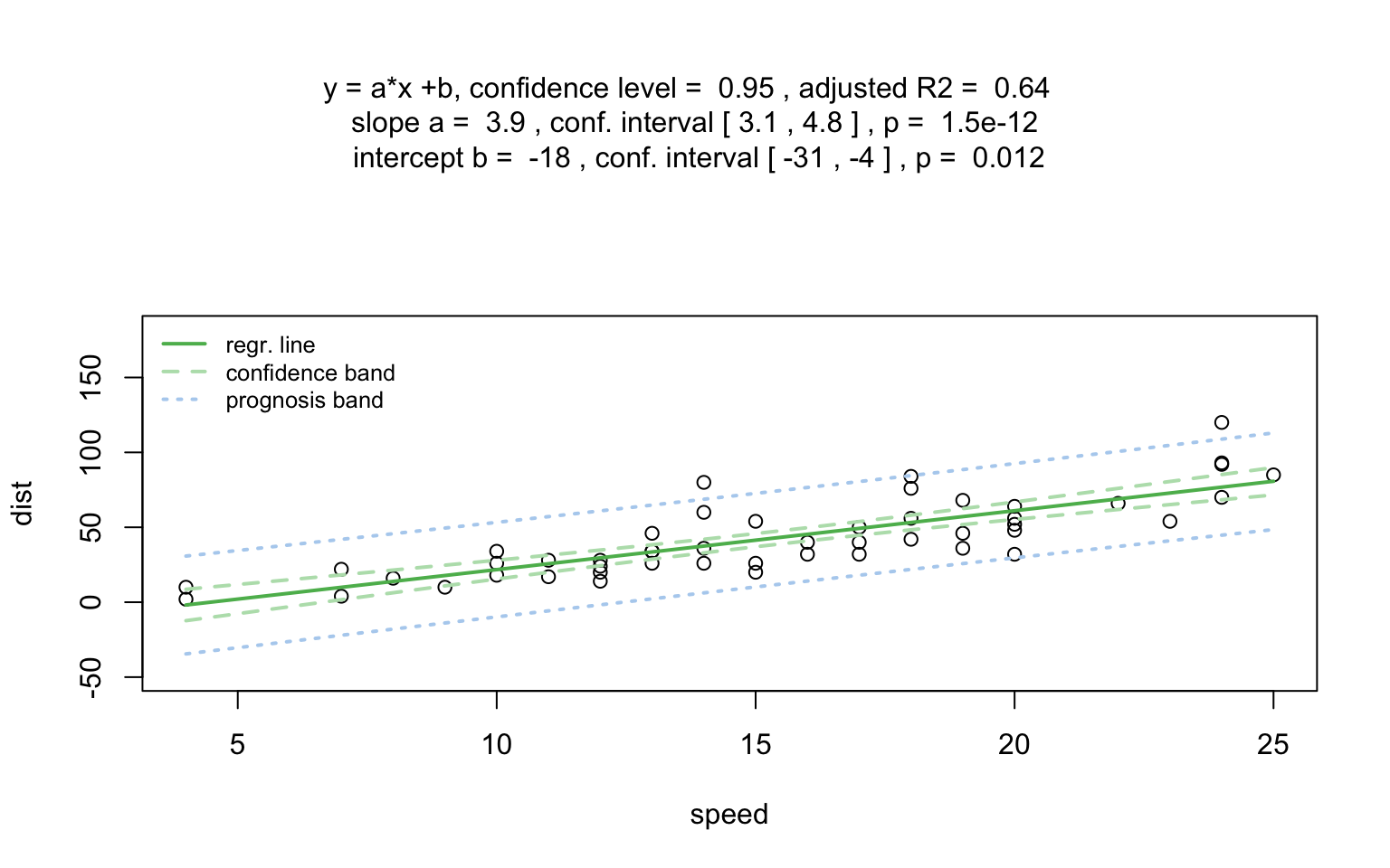
Increasing the confidence level conf.level from the
default 0.95 to 0.99 leads two wider confidence and prediction
bands:
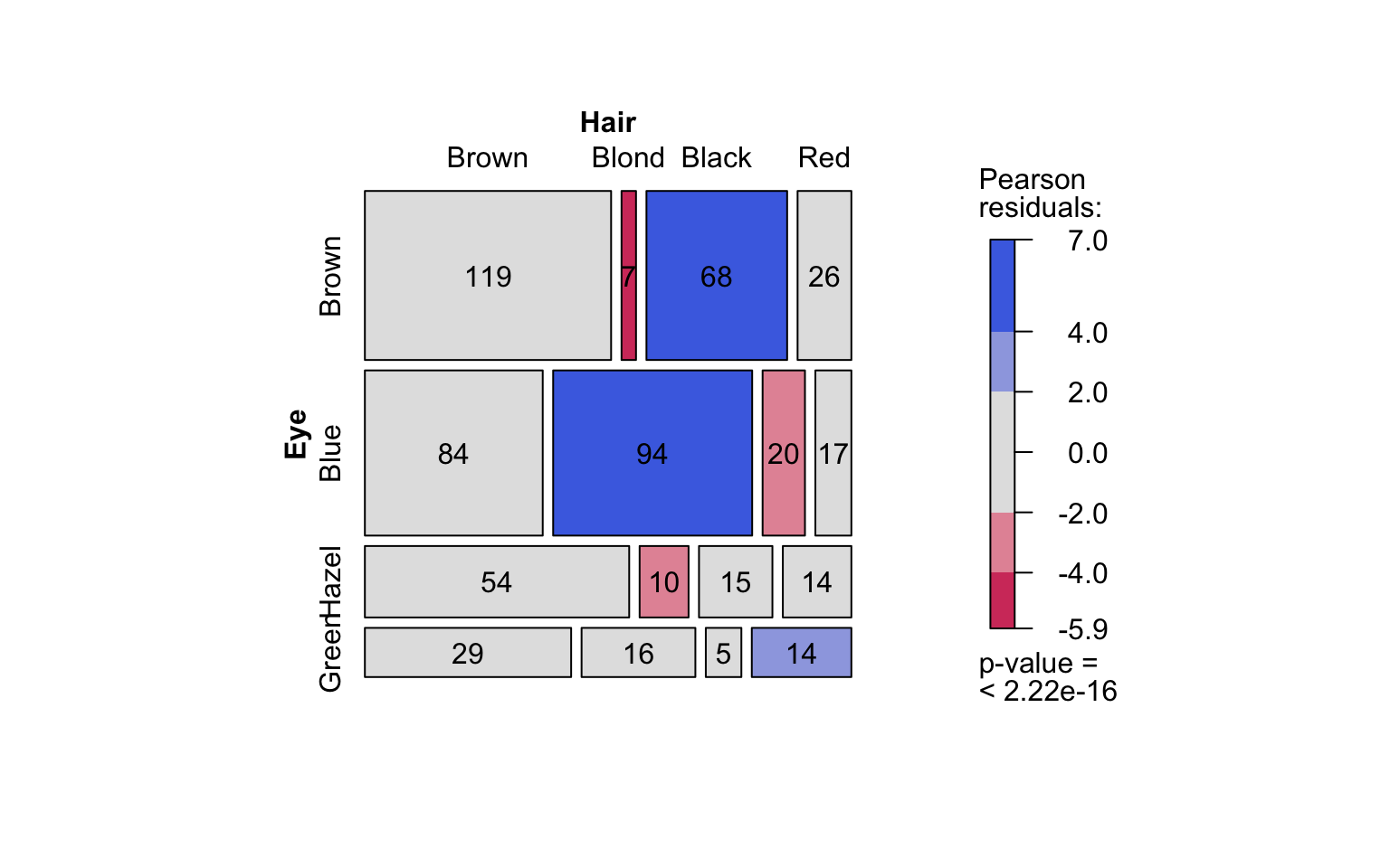
Count data sets are often presented as multidimensional arrays, so -
called contingency tables, whereas visstat() requires a
data.frame with a column structure. Arrays can be
transformed to this column wise structure with the helper function
counts_to_cases():
hair_eye_color_df <- counts_to_cases(as.data.frame(HairEyeColor))
visstat(hair_eye_color_df$Eye, hair_eye_color_df$Hair)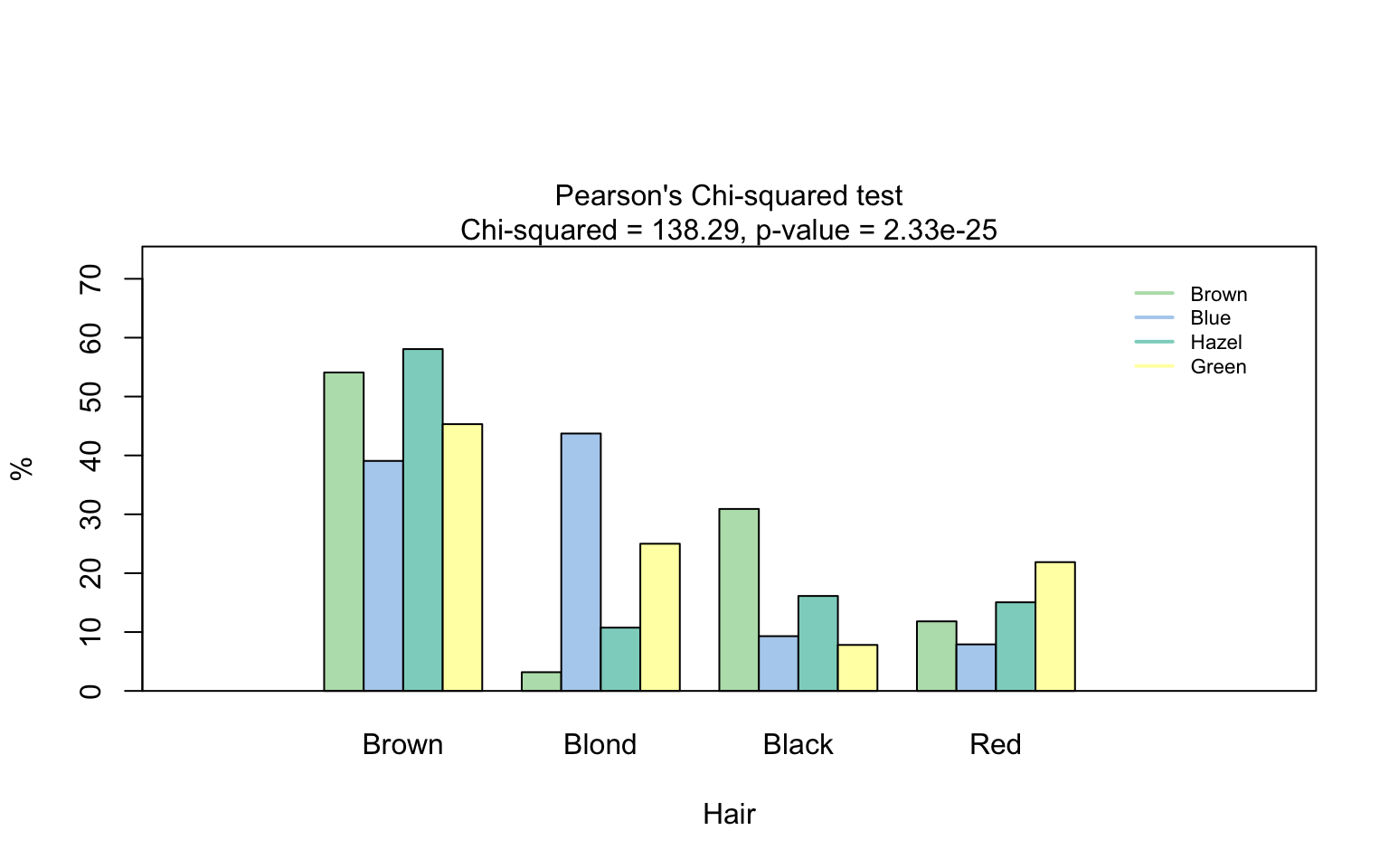
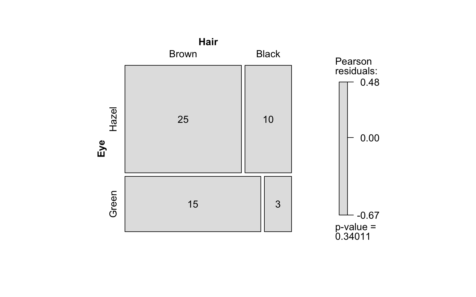
hair_eye_color_male <- HairEyeColor[, , 1]
# Slice out a 2 by 2 contingency table
black_brown_hazel_green_male <- hair_eye_color_male[1:2, 3:4]
# Transform to data frame
black_brown_hazel_green_male <- counts_to_cases(as.data.frame(black_brown_hazel_green_male))
# Fisher test
fisher_stats <- visstat(black_brown_hazel_green_male$Eye,black_brown_hazel_green_male$Hair)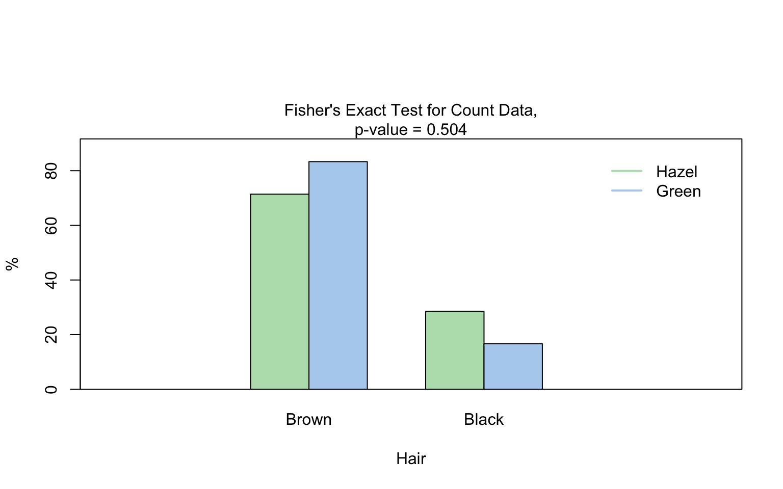
The choice of statistical tests depends on whether the data of the selected columns are numeric or categorical, the number of levels in the categorical variable, and the distribution of the data. The function prioritizes interpretable visual output and tests that remain valid under the the following decision logic:
When the response is numeric and the predictor is categorical, a statistical hypothesis test of central tendencies is selected.
If the categorical predictor has exactly two levels, Welch’s t -
test (t.test()), is applied whenever both groups contain
more than 30 observations, with the validity of the test supported by
the approximate normality of the sampling distribution of the mean under
the central limit theorem [@Rasch:2011vl @Lumley2002dsa]. For smaller samples,
group - wise normality is assessed using the Shapiro - Wilk test
(shapiro.test()) at the significance levelα. If
both groups are found to be approximately normally distributed according
to the Shapiro - Wilk test, Welch’s t-test is applied; otherwise, the
Wilcoxon rank-sum test (wilcox.test()) is used.
For predictors with more than two levels, an ANOVA model
(aov()) is initially fitted. The normality of residuals is
evaluated using both the Shapiro–Wilk test (shapiro.test())
and the Anderson–Darling test (ad.test()); residuals are
considered approximately normal if at least one of the two tests yields
a result exceeding the significance threshold α. If this
condition is met, Bartlett’s test (bartlett.test()) is then
used to assess homoscedasticity. When variances are homogeneous
(p > α), ANOVA is applied with Tukey’s HSD
(TukeyHSD()) for post-hoc comparison. If variances differ
significantly (p ≤ α), Welch’s one - way test
(oneway.test()) is used, also followed by Tukey’s HSD. If
residuals are not normally distributed according to both tests
(p ≤ α), the Kruskal-Wallis test
(kruskal.test()) is selected, followed by pairwise Wilcoxon
tests (pairwise.wilcox.test()). A graphical overview of the
decision logic used is provided in below figure.
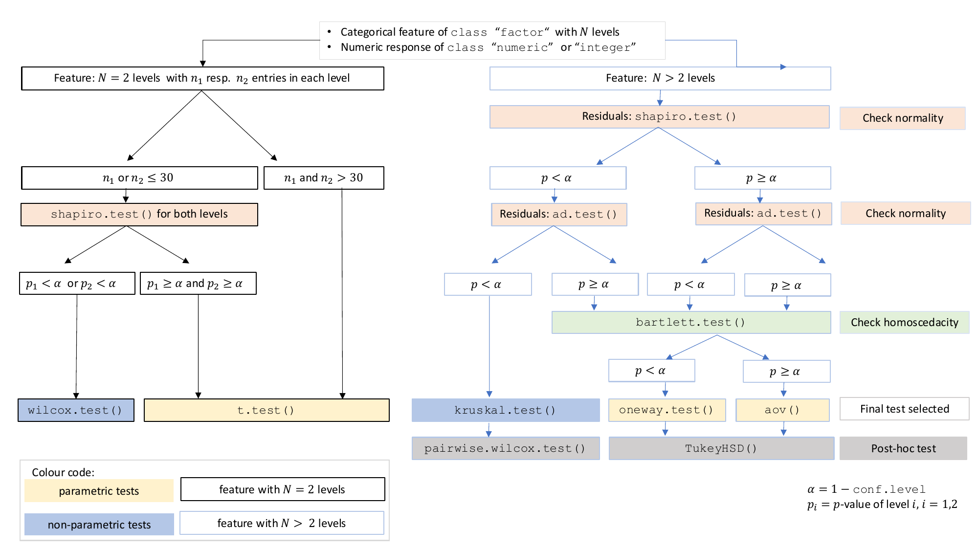
Decision tree used to select the appropriate statistical test for a categorical predictor and numeric response, based on the number of factor levels, normality, and homoscedasticity.
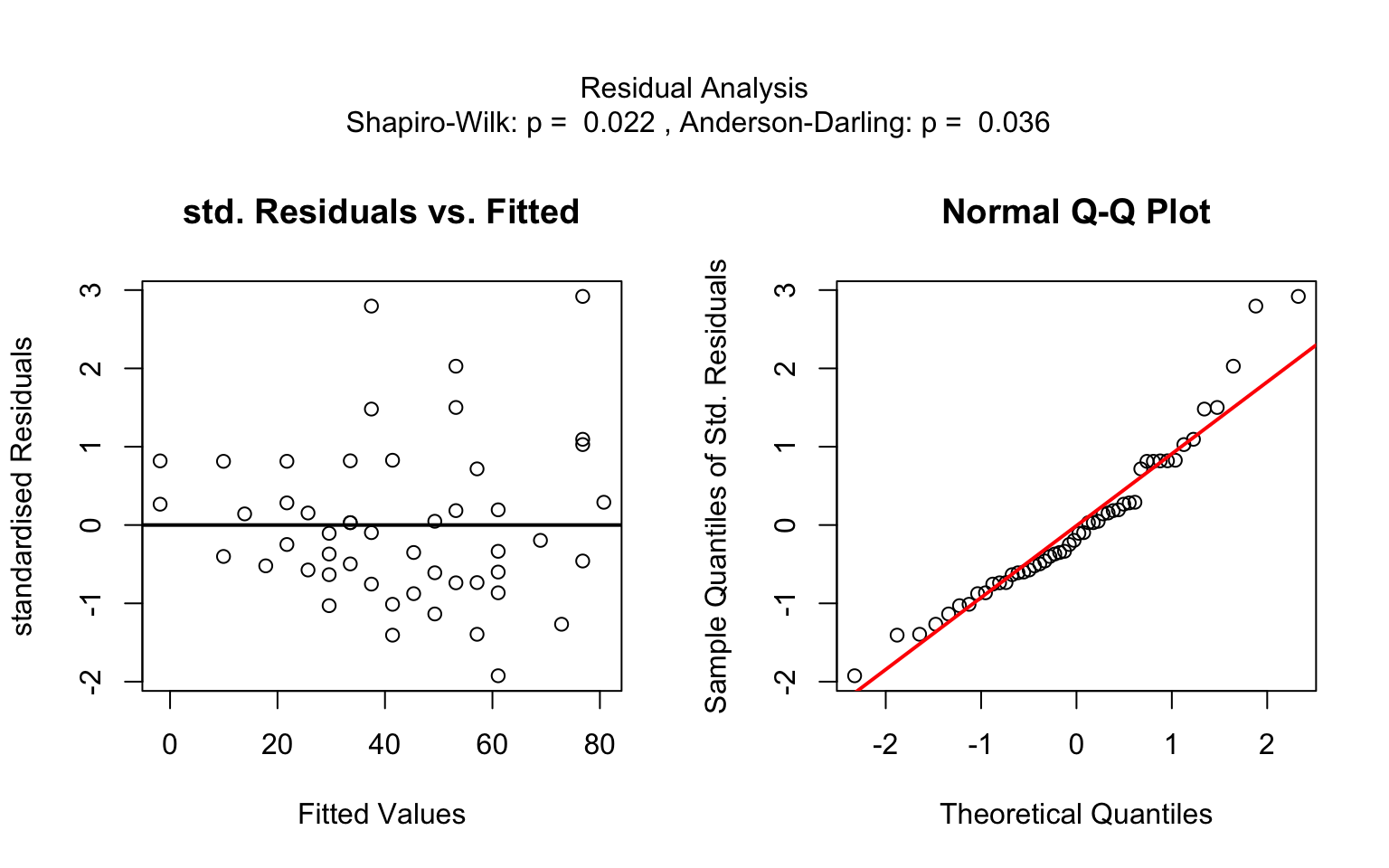
When both the response and predictor are numeric, a simple linear
regression model (lm()) is fitted and analysed in detail,
including residual diagnostics, formal tests, and the plotting of fitted
values with confidence bands. Note that only one explanatory variable is
allowed, as the function is designed for two-dimensional
visualisation.
When both variables are categorical, no direction is assumed (though
one is still referred to as the for consistency). visstat()
tests the null hypothesis that both variables are independent using
either chisq.test() or fisher.test(). The
choice of test is based on Cochran’s rule [@Cochran], which advises that
theχ2approximation is reliable only if no expected
cell count is zero and no more than 20 percent of cells have expected
counts below 5.
For a more detailed description of the underlying decision logic see
vignette("visStatistics")The main purpose of this package is a decision-logic based automatic
visualisation of statistical test results. Therefore, except for the
user-adjustable conf.level parameter, all statistical tests
are applied using their default settings from the corresponding base R
functions. As a consequence, paired tests are currently not supported
and visstat() does not allow to study interactions terms
between the different levels of an independent variable in an analysis
of variance. Focusing on the graphical representation of tests, only
simple linear regression is implemented, as multiple linear regressions
cannot be visualised.
t.test(), wilcox.test(),
aov(), oneway.test(),
kruskal.test()
shapiro.test() and ad.test()
bartlett.test()
TukeyHSD() (used following aov()and
oneway.test())pairwise.wilcox.test() (used following
kruskal.test())When both the response and predictor are numerical, a simple linear
regression model is fitted:lm()
Note that multiple linear regression models are not implemented, as the package focuses on the visualisation of data, not model building. ### Categorical response and categorical predictor
When both variables are categorical, visstat() tests the
null hypothesis of independence using one of the
following:-chisq.test() (default for larger samples) -
fisher.test() (used for small expected cell counts based on
Cochran’s rule)