Estimate one or two cutpoints of a variable of interest in the multivariable context of survival data or time-to-event data
Visualise the cutpoint estimation process using contour plots, index plots, and spline plots
Estimate cutpoints based on the assumption of a U-shaped or inverted U-shaped relationship between the predictor and the hazard ratio
You can install the development version of cutpoint from GitHub with:
# install.packages("pak")
pak::pak("jan-por/cutpoint")The R package cutpoint is used to determine cutpoints of
variables, such as biomarkers, in the multivariable context of survival
or time-to-event analyses. These cutpoints are applied to form groups
with different probabilities of an event occurring.
For example, in medical research, cutpoints of biomarkers are formed
to classify patients into different risk groups regarding survival in
tumor diseases. Using the R package cutpoint, it is
possible to estimate one or two cutpoints for categorising a variable of
interest, while taking other relevant variables into account. Thus, it
is possible, for instance in the medical context, not only to estimate a
cutpoint based on a single biomarker but also to consider other
biomarkers or baseline characteristics.
The R packet cutpoint allows for a combined approach to determining cutpoints, particularly through numerical calculations and visual examination of different plots according to their functional forms.
For the numerical calculation, either the AIC (Akaike Information Criterion) or the LRT (Likelihood-Ratio Test statistic) is used to estimate the cutpoint in the context of Cox regression. The Likelihood Ratio Test statistic is calculated by taking the scaled difference between the log-likelihoods of the model and the null model’s log-likelihoods. Details on the methods can be found in the article by Govindarajulu, U., & Tarpey, T. (2022). Optimal partitioning for the proportional hazards model. Journal of Applied Statistics, 49(4), 968–987. doi:10.1080/02664763.2020.1846690
The cp_est function estimates one or two cutpoints for a
biomarker. The argument ushape enables cutpoints to be
estimated assuming the splines plot displays a U-shaped or inverted
U-shaped curve. The symtail argument allows for the
estimation of two cutpoints, ensuring that the two outer tails represent
groups of approximately the same size.
Estimate one cutpoint of the variable biomarker under consideration of two other covariates.
For this example, the dataset data1, included in the
R-package cutpoint, is used. It has 100 observations and
contains the variables:
Because one cutpoint should be estimated, the argument
nb_of_cp is set to 1. (nb_of_cp = 1)
For the other arguments, their default settings are used:
Min. group size in % bandwidth = 0.1
Estimation type est_type = "AIC"
Cutpoint variable as strata in Cox model?
cpvar_strata = FALSE (not as strata)
Symmetric tails symtails = FALSE
Cutpoints for u-shape ushape = FALSE
library(cutpoint)
cpobj <- cp_est(
   cpvarname = "biomarker",
   covariates = c("covariate_1", "covariate_2"),
   data = data1,
   nb_of_cp = 1
)The output displays the primary settings and the cutpoint:
#>
#> Approx. remaining time for estimation: 1 seconds
#> --------------------------------------------------------------------
#> SETTINGS:
#>  Cutpoint-variable                    =  biomarker
#>  Number of cutpoints   (nb_of_cp)     =  1
#>  Min. group size in %  (bandwith)     =  0.1
#>  Estimation type       (est_type)     =  AIC
#>  CP-variable as strata (cpvar_strata) =  FALSE
#>  Symmetric tails       (symtails)     =  FALSE   (is set to FALSE if nb_of_cp = 1)
#>  Cutpoints for u-shape (ushape)       =  FALSE   (is set to FALSE if nb_of_cp = 1)
#> --------------------------------------------------------------------
#> Covariates or factors are:
#>   covariate_1 covariate_2
#> --------------------------------------------------------------------
#> Minimum group size is 10 (10% of sample size in original dataset, N = 100)
#> --------------------------------------------------------------------
#> Number of cutpoints searching for: 1
#> Cutpoint: biomarker ≤ 89
#> -----------------------------------------------------------------
#> Group size in relation to valid data of biomarker in original data set
#>  Total:                N = 100 (100%)
#>  Group A (lower part): n = 12 (12%)
#>  Group B (upper part): n = 88 (88%)
The argument bandwidth can change the minimum group
sizes and may lead to different cutpoint estimates.
Other cutpoints may be estimated if no covariates
(covariates = NULL) are included in the cutpoint
search:
library(cutpoint)
cpobj <- cp_est(
   cpvarname = "biomarker",
   covariates = NULL,
   data = data1,
   nb_of_cp = 1
)With covariates, the cutpoint was ≤ 89; without covariates the cutpoint is ≤ 137:
#>
#> Approx. remaining time for estimation: 0 seconds
#> --------------------------------------------------------------------
#> SETTINGS:
#>  Cutpoint-variable                    =  biomarker
#>  Number of cutpoints   (nb_of_cp)     =  1
#>  Min. group size in %  (bandwith)     =  0.1
#>  Estimation type       (est_type)     =  AIC
#>  CP-variable as strata (cpvar_strata) =  FALSE
#>  Symmetric tails       (symtails)     =  FALSE   (is set to FALSE if nb_of_cp = 1)
#>  Cutpoints for u-shape (ushape)       =  FALSE   (is set to FALSE if nb_of_cp = 1)
#> --------------------------------------------------------------------
#> No covariates were selected
#> --------------------------------------------------------------------
#> Minimum group size is 10 (10% of sample size in original dataset, N = 100)
#> --------------------------------------------------------------------
#> Number of cutpoints searching for: 1
#> Cutpoint: biomarker ≤ 137
#> -----------------------------------------------------------------
#> Group size in relation to valid data of biomarker in original data set
#>  Total:                N = 100 (100%)
#>  Group A (lower part): n = 29 (29%)
#> Group B (upper part): n = 71 (71%)The cp_value_plot and cp_splines_plot
functions are utilised to choose the appropriate cutpoints.
The default plot of the function cp_est is a
covariate-adjusted splines plot with different degrees of freedom. This
plot can also be generated using the function
cp_splines_plot, which enables the creation of
covariate-adjusted or non-adjusted splines plots.
cp_splines_plot(cpobj, show_splines = TRUE, adj_splines = TRUE)
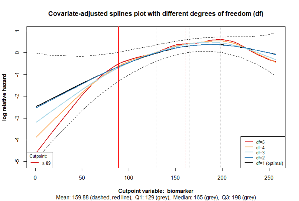
The cutpoint is shown as a vertical red line, while the dashed red
line represents the mean of the variable of interest. The first
quartile, median, and third quartile are indicated in grey. The lines,
which are based on different degrees of freedom should facilitate in
determining, whether misspecification or overfitting occurs. The former
example does not appear to be one of those. Therefore the function
cp_splines_plot can be used with the argument
show_splines = FALSE to obtain a clearer illustration:
cp_splines_plot(cpobj, show_splines = FALSE, adj_splines = TRUE)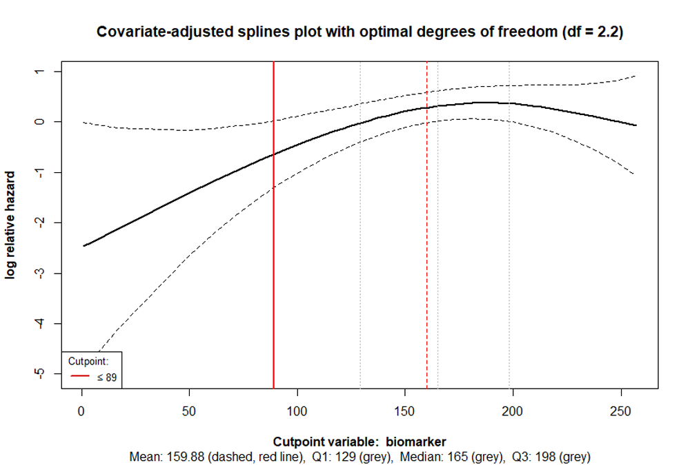
The function cp_value_plot enables the creation of
contour plots and index plots from a cpobj Object. The AIC
values of the cutpoint estimation process or the Likelihood Ratio Test
statistic (LRT) statistic can be used for this.
Example: Estimate two cutpoints of the variable biomarker under consideration of two other covariates:
library(cutpoint)
cpobj <- cp_est(
   cpvarname = "biomarker",
   covariates = c("covariate_1", "covariate_2"),
   data = data1,
   nb_of_cp = 2
   )
Call plot:
cp_value_plot(cpobj, plotvalues = "AIC", plottype2cp = "contour")
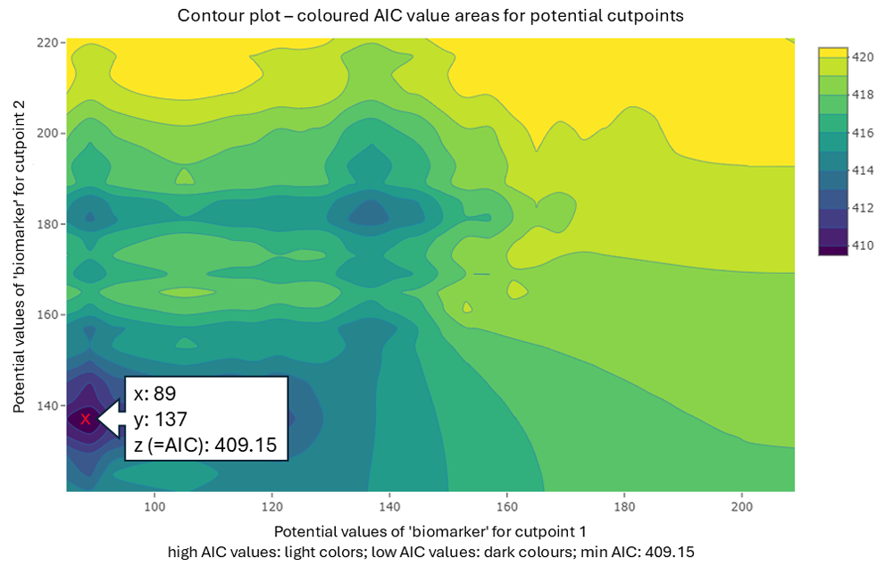
The x-axis and y-axis represent potential cutpoint values, while the AIC values from the estimation process are coloured. The lowest AIC values are shown in dark colours and may indicate potential cutpoints. The estimated cutpoints are: Cutpoint 1 ≤ 89 and Cutpoint 2 ≤ 137 (marked).
The next plot (Figure 4) illustrates another example of a biomarker from
another virtual dataset, identifying two possible cutpoint combinations.
The AIC values differ only slightly (3558.3 vs 3558.2). From a
statistical point of view, both cutpoint combinations may be acceptable.
However, perhaps one of the two options is more reasonable from a
scientific perspective. Therefore, it is beneficial to utilise the
output in the console and examine the plots.
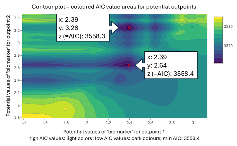
The smaller the bandwidth (minimum group size per group),
the more precise and meaningful the contour plots can be
interpreted.
The index plot below is based on the same example used for Figure 4.
The x-axis represents the index of all possible combinations for the two
cutpoints being searched for. In this case, there are more than 60.000.
As Figure 4 already shows, and Figure 5 indicates, two areas have lower
AIC values (marked).
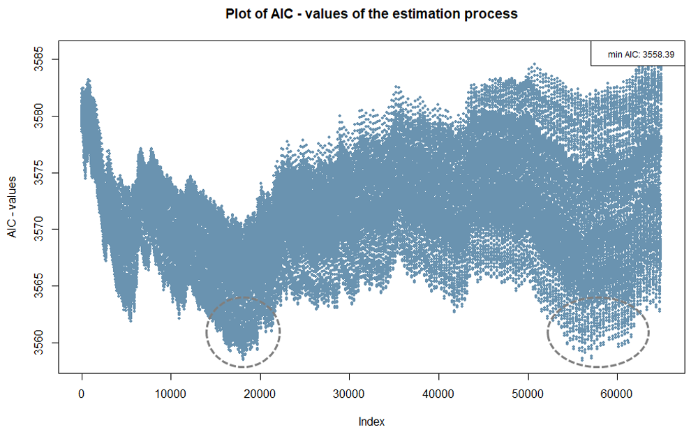
Index plots that do not show clear areas with extreme values, as
illustrated in Figure 5, suggest that a real cutpoint may not exist in
the data. However, even if there is no true cutpoint in the data, it is
often possible to establish cutpoints, allowing for the formation of
groups with different probabilities of an event occurring.
The function cp_est has the argument ushape
with two possible characteristics: TRUE or
FALSE. If ushape = TRUE, the cutpoints are
estimated based on the assumption of a U-shaped or inverted U-shaped
relationship between the predictor and the hazard ratio.
ushape = TRUE is only achievable when two cutpoints are
searched for.
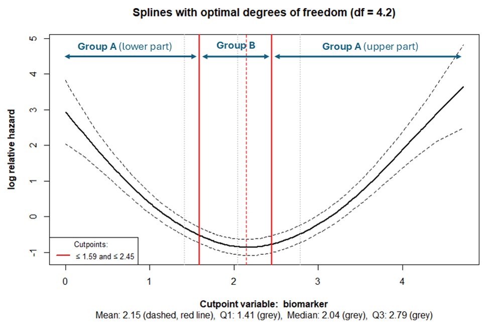
The outer tails belong to the same risk group (lower-, and upper part
of Group A), while the midsection constitutes a different risk group
(Group B) (see Figure 6). The outer tails must not necessarily be the
same size. If they are to be of approximately the same size, the
argument symtails has been set to
symtails = TRUE.
Example: Estimate two cutpoints of the variable biomarker under consideration of one covariate:
cpobj <- cp_est(
  cpvarname    = "biomarker",
  covariates   = c("covariate_1"),
  data         = data2_ushape,
  nb_of_cp     = 2,
  bandwith     = 0.2,
  ushape       = TRUE,
  symtails     = FALSE,
  plot_splines = FALSE
)#>
#> Approx. remaining time for estimation: 9 seconds
#> --------------------------------------------------------------------
#> SETTINGS:
#> Cutpoint-variable = biomarker
#> Number of cutpoints (nb_of_cp) = 2
#> Min. group size in % (bandwith) = 0.2
#> Estimation type (est_type) = AIC
#> CP-variable as strata (cpvar_strata) = FALSE
#> Symmetric tails (symtails) = FALSE (is set to FALSE if nb_of_cp = 1)
#> Cutpoints for u-shape (ushape) = TRUE (is set to FALSE if nb_of_cp = 1)
#> --------------------------------------------------------------------
#> Covariates or factors are:
#> covariate_1
#> --------------------------------------------------------------------
#> Minimum group size is 40 (20% of sample size in original dataset, N = 200)
#> --------------------------------------------------------------------
#> Number of cutpoints searching for: 2
#> 1.Cutpoint: biomarker ≤ 1.589527
#> 2.Cutpoint: biomarker ≤ 2.445578
#> -----------------------------------------------------------------
#> Group size in relation to valid data of biomarker in original data set:
#> Total: N = 200 (100%)
#> Group A (lower part): n = 59 (29.5%)
#> Group B (middle part): n = 65 (32.5%)
#> Group A (upper part): n = 76 (38%)
If a U-shaped or inverted U-shaped relationship exists, it can be evaluated using the spline plot:
cp_splines_plot(cpobj, show_splines = FALSE)
To report a bug, please open an issue
Porthun, J. (2025). Estimate cutpoints in the multivariable context of survival or time-to-event data. cutpoint R package. Retrieved from https://github.com/jan-por/cutpoint
Jan Porthun | NTNU Norwegian University of Science and Technology