The goal of the move2 package is to facilitate handling
movement data by creating the move2 class that extents the
functionality of the sf package. It facilitates import of
animal movement data from movebank.
The move2 package is designed as a successor to the
move package, but improves in speed and functionality by
being redesigned from the ground up. More documentation can be found on
the website.
The most recent released version of move2 can be
installed directly from CRAN:
install.packages("move2")You can also install the development version of move2
like so:
devtools::install_git('https://gitlab.com/bartk/move2.git')By using units it is possible to track changes through analysis, note that ggplot directly has the correct units on the y axis
require(units)
require(dplyr)
require(ggplot2)
require(move2)
require(rnaturalearth)
track <- movebank_download_study("Galapagos Albatrosses",
  sensor_type_id = "gps"
)
track
#> A <move2> with `track_id_column` "individual_local_identifier" and
#> `time_column` "timestamp"
#> Containing 28 tracks lasting on average 37.1 days in a
#> Simple feature collection with 16414 features and 18 fields (with 386 geometries empty)
#> Geometry type: POINT
#> Dimension:     XY
#> Bounding box:  xmin: -91.3732 ymin: -12.79464 xmax: -77.51874 ymax: 0.1821983
#> Geodetic CRS:  WGS 84
#> # A tibble: 16,414 × 19
#>   sensor_type_id individual_local_identifier eobs_battery_voltage
#>          <int64> <fct>                                       [mV]
#> 1            653 4264-84830852                               3686
#> 2            653 4264-84830852                               3701
#> 3            653 4264-84830852                               3701
#> 4            653 4264-84830852                               3691
#> # ℹ 16,410 more rows
#> # ℹ 16 more variables: eobs_fix_battery_voltage [mV],
#> #   eobs_horizontal_accuracy_estimate [m], eobs_key_bin_checksum <int64>,
#> #   eobs_speed_accuracy_estimate [m/s], eobs_start_timestamp <dttm>,
#> #   eobs_status <ord>, eobs_temperature [°C], eobs_type_of_fix <fct>,
#> #   eobs_used_time_to_get_fix [s], ground_speed [m/s], heading [°],
#> #   height_above_ellipsoid [m], timestamp <dttm>, visible <lgl>, …
#> First 4 track features:
#> # A tibble: 28 × 52
#>   deployment_id  tag_id individual_id animal_life_stage attachment_type
#>         <int64> <int64>       <int64> <fct>             <fct>
#> 1       2911170 2911124       2911090 adult             tape
#> 2       2911150 2911126       2911091 adult             tape
#> 3       2911167 2911127       2911092 adult             tape
#> 4       2911168 2911129       2911093 adult             tape
#> # ℹ 24 more rows
#> # ℹ 47 more variables: deployment_comments <chr>, deploy_on_timestamp <dttm>,
#> #   duty_cycle <chr>, deployment_local_identifier <fct>,
#> #   manipulation_type <fct>, study_site <chr>, tag_readout_method <fct>,
#> #   sensor_type_ids <chr>, capture_location <POINT [°]>,
#> #   deploy_on_location <POINT [°]>, deploy_off_location <POINT [°]>,
#> #   individual_comments <chr>, individual_local_identifier <fct>, …
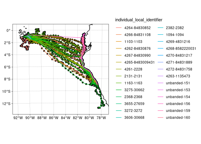
ggplot() +
  geom_sf(data = ne_coastline(returnclass = "sf", 10)) +
  theme_linedraw() +
  geom_sf(data = track) +
  geom_sf(data = mt_track_lines(track), aes(color = `individual_local_identifier`)) +
  coord_sf(
    crs = sf::st_crs("+proj=aeqd +lon_0=-83 +lat_0=-6 +units=km"),
    xlim = c(-1000, 600),
    ylim = c(-800, 700)
  )
#> In total 386 empty location records are removed before summarizing.
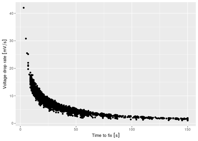
track %>%
  ggplot() +
  geom_point(aes(
    x = `eobs_used_time_to_get_fix`,
    y = (`eobs_battery_voltage` - `eobs_fix_battery_voltage`) / `eobs_used_time_to_get_fix`
  )) +
  xlab("Time to fix") +
  ylab("Voltage drop rate")
#> Warning: The `scale_name` argument of `continuous_scale()` is deprecated as of ggplot2
#> 3.5.0.
#> This warning is displayed once every 8 hours.
#> Call `lifecycle::last_lifecycle_warnings()` to see where this warning was
#> generated.
Several other packages exist for dealing with movement data. For an
overview see the CRAN task view. Here we
make a quick comparison to some other packages that define movement
datasets and the differences to move2:
move: The move package is based on
sp and therefore the S4 classes. This class
system is very capable but it sometimes results in the data being more
difficult to handle. Furthermore as sf improves on
sp move2 will be able to improve in
speed.sftrack: Does not include trajectory information.
Furthermore the sft_group attribute is quite large (in
memory due to being a character) and relatively slow.amt/trajr/ctmm: These do not
extend a spatial class meaning other spatial functions do not work on
these trajectories. Furthermore these objects do not keep track of
trajectory level information (e.g. sex, data of birth & capture
location).Compared to the other packages move2 tries to be
flexible enough that it is easy to use in other software but still
retains the formal properties and all meta data of trajectories.
Therefore we avoid more complicated data structures (e.g. Kranstauber et
al, 2011).
Currently the move2 package focuses on core
functionality, ideas for additional packages exist:
moveAcc/moveIMU: probably using
vctrs/pillar for storing bursts of
acceleration or orientation data.moveUd: for example Brownian bridgesmoveSim: for simulation trajectoriesmoveShiny: for simple quick apps using shiny modules
for visualizing and exploring trajectoriesmove2There are ideas for additional functionality they are not directly implemented but recorded here to keep them on the radar. Specific suggestions or information what is used are welcome.
filter_duplicate_locations_minimal_travelfilter_minimal_travel: Minimally x meter travel between
locationsfilter_minimal_distance: Minimally x meter distance
between locationsfilter_outlier_quick_return: Combination of ~180 degree
turns, high speed and comparable distances?By installing the package todor it is possible to find
all to-dos as markers through the rstudio addins menu, or
run todor::todor_package_addin(). Furthermore we use
precommit to validate code before committing. Testing is
done through testthat.
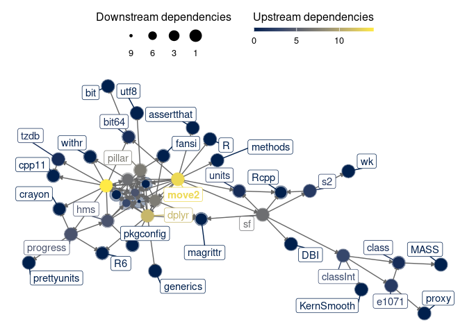
depgraph::plot_dependency_graph(".", suggests = FALSE)