ggmap is an R package that makes it easy to retrieve raster map tiles from popular online mapping services like Google Maps, Stadia Maps, and OpenStreetMap, and plot them using the ggplot2 framework.
Stadia Maps offers map tiles in several styles, including updated tiles from Stamen Design. An
API key is required, but no credit card is necessary to sign up and there is a
free tier for non-commercial use. Once you have your API key, invoke the
registration function:
register_stadiamaps("YOUR-API-KEY", write = FALSE). Note
that setting write = TRUE will update your
~/.Renviron file by replacing/adding the relevant line. If
you use the former, know that you’ll need to re-do it every time you
reset R.
Your API key is private and unique to you, so be careful not to share it online, for example in a GitHub issue or saving it in a shared R script file. If you share it inadvertently, just go to client.stadiamaps.com, delete your API key, and create a new one.
library("ggmap")
#  Loading required package: ggplot2
#  ℹ Google's Terms of Service: <https://mapsplatform.google.com>
#    Stadia Maps' Terms of Service: <https://stadiamaps.com/terms-of-service/>
#    OpenStreetMap's Tile Usage Policy: <https://operations.osmfoundation.org/policies/tiles/>
#  ℹ Please cite ggmap if you use it! Use `citation("ggmap")` for details.

us <- c(left = -125, bottom = 25.75, right = -67, top = 49)
get_stadiamap(us, zoom = 5, maptype = "alidade_smooth") |> ggmap()
#  ℹ © Stadia Maps © Stamen Design © OpenMapTiles © OpenStreetMap contributors.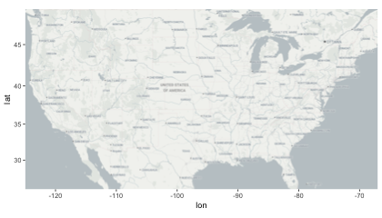
Use qmplot() in the same way you’d use
qplot(), but with a map automatically added in the
background:
library("dplyr", warn.conflicts = FALSE)
library("forcats")

# define helper
`%notin%` <- function(lhs, rhs) !(lhs %in% rhs)

# reduce crime to violent crimes in downtown houston
violent_crimes <- crime |>
  filter(
    offense %notin% c("auto theft", "theft", "burglary"),
    between(lon, -95.39681, -95.34188),
    between(lat, 29.73631, 29.78400)
  ) |>
  mutate(
    offense = fct_drop(offense),
    offense = fct_relevel(offense, c("robbery", "aggravated assault", "rape", "murder"))
  )

# use qmplot to make a scatterplot on a map
qmplot(lon, lat, data = violent_crimes, maptype = "stamen_toner_lite", color = I("red"))
#  ℹ Using `zoom = 14`
#  ℹ © Stadia Maps © Stamen Design © OpenMapTiles © OpenStreetMap contributors.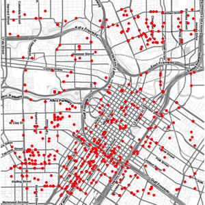
Often qmplot() is easiest because it automatically
computes a nice bounding box for you without having to pre-compute it
for yourself, get a map, and then use ggmap(map) in place
of where you would ordinarily (in a ggplot2
formulation) use ggplot(). Nevertheless, doing it yourself
is more efficient. In that workflow you get the map first (and you can
visualize it with ggmap()):
bbox <- make_bbox(lon, lat, data = violent_crimes)
map <- get_stadiamap( bbox = bbox, maptype = "stamen_toner_lite", zoom = 14 )
#  ℹ © Stadia Maps © Stamen Design © OpenMapTiles © OpenStreetMap contributors.
ggmap(map)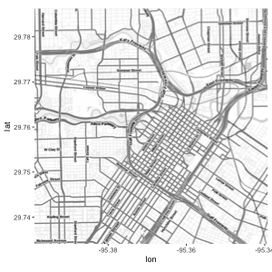
And then you layer on geoms/stats as you would with
ggplot2. The only difference is that (1) you need to
specify the data arguments in the layers and (2) the
spatial aesthetics x and y are set to
lon and lat, respectively. (If they’re named
something different in your dataset, just put
mapping = aes(x = longitude, y = latitude)), for
example.)
ggmap(map) +
  geom_point(data = violent_crimes, color = "red")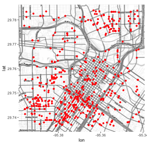
With ggmap you’re working with
ggplot2, so you can add in other kinds of layers, use
patchwork,
etc. All the ggplot2 geom’s are available. For example,
you can make a contour plot with geom = "density2d":
library("patchwork")
library("ggdensity")

robberies <- violent_crimes |> filter(offense == "robbery")

points_map <- ggmap(map) + geom_point(data = robberies, color = "red")

# warnings disabled
hdr_map <- ggmap(map) +
  geom_hdr(
    aes(lon, lat, fill = after_stat(probs)), data = robberies,
    alpha = .5
  ) +
  geomtextpath::geom_labeldensity2d(
    aes(lon, lat, level = after_stat(probs)),
    data = robberies, stat = "hdr_lines", size = 3, boxcolour = NA
  ) +
  scale_fill_brewer(palette = "YlOrRd") +
  theme(legend.position = "none")

(points_map + hdr_map) &
  theme(axis.title = element_blank(), axis.text = element_blank(), axis.ticks = element_blank())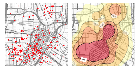
Faceting works, too:
ggmap(map, darken = .3) +
  geom_point(
    aes(lon, lat), data = violent_crimes,
    shape = 21, color = "gray25", fill = "yellow"
  ) +
  facet_wrap(~ offense, nrow = 1) +
  theme(axis.title = element_blank(), axis.text = element_blank(), axis.ticks = element_blank())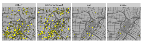
Google Maps can be used just as easily. However, since Google Maps use a center/zoom specification, their input is a bit different:
(map <- get_googlemap("waco texas", zoom = 12))
#  ℹ <https://maps.googleapis.com/maps/api/staticmap?center=waco%20texas&zoom=12&size=640x640&scale=2&maptype=terrain&key=xxx>
#  ℹ <https://maps.googleapis.com/maps/api/geocode/json?address=waco+texas&key=xxx>
#  1280x1280 terrain map image from Google Maps; use `ggmap::ggmap()` to plot it.
ggmap(map)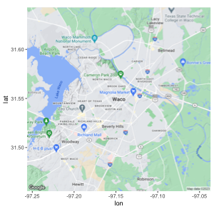
Moreover, you can get various different styles of Google Maps with ggmap (just like Stadia Maps):
get_googlemap("waco texas", zoom = 12, maptype = "satellite") |> ggmap()
get_googlemap("waco texas", zoom = 12, maptype = "hybrid") |> ggmap()
get_googlemap("waco texas", zoom = 12, maptype = "roadmap") |> ggmap()
Google’s geocoding and reverse geocoding API’s are available through
geocode() and revgeocode(), respectively:
geocode("1301 S University Parks Dr, Waco, TX 76798")
#  ℹ <https://maps.googleapis.com/maps/api/geocode/json?address=1301+S+University+Parks+Dr,+Waco,+TX+76798&key=xxx>
#  # A tibble: 1 × 2
#      lon   lat
#    <dbl> <dbl>
#  1 -97.1  31.6
revgeocode(c(lon = -97.1161, lat = 31.55098))
#  ℹ <https://maps.googleapis.com/maps/api/geocode/json?latlng=31.55098,-97.1161&key=xxx>
#  Warning: Multiple addresses found, the first will be returned:
#  !   1301 S University Parks Dr, Waco, TX 76706, USA
#  !   55 Baylor Ave, Waco, TX 76706, USA
#  !   1437 S University Parks Dr, Waco, TX 76706, USA
#  !   HV2M+9H Waco, TX, USA
#  !   Bear Trail, Waco, TX 76706, USA
#  !   Robinson, TX 76706, USA
#  !   Waco, TX, USA
#  !   McLennan County, TX, USA
#  !   Texas, USA
#  !   United States
#  [1] "1301 S University Parks Dr, Waco, TX 76706, USA"
Note: geocode() uses Google’s Geocoding API to
geocode addresses. Please take care not to disclose sensitive
information. Rundle, Bader,
and Moody (2022) have considered this issue and suggest various
alternative options for such data.
There is also a mutate_geocode() that works similarly to
dplyr’s
mutate() function:
tibble(address = c("white house", "", "waco texas")) |>
  mutate_geocode(address)
#  ℹ <https://maps.googleapis.com/maps/api/geocode/json?address=white+house&key=xxx>
#  ℹ <https://maps.googleapis.com/maps/api/geocode/json?address=waco+texas&key=xxx>
#  # A tibble: 3 × 3
#    address         lon   lat
#    <chr>         <dbl> <dbl>
#  1 "white house" -77.0  38.9
#  2 ""             NA    NA
#  3 "waco texas"  -97.1  31.6
Treks use Google’s routing API to give you routes
(route() and trek() give slightly different
results; the latter hugs roads):
trek_df <- trek("houson, texas", "waco, texas", structure = "route")
#  ℹ <https://maps.googleapis.com/maps/api/directions/json?origin=houson,+texas&destination=waco,+texas&key=xxx&mode=driving&alternatives=false&units=metric>
qmap("college station, texas", zoom = 8) +
  geom_path(
    aes(x = lon, y = lat),  colour = "blue",
    size = 1.5, alpha = .5,
    data = trek_df, lineend = "round"
  )
#  ℹ <https://maps.googleapis.com/maps/api/staticmap?center=college%20station,%20texas&zoom=8&size=640x640&scale=2&maptype=terrain&language=en-EN&key=xxx>
#  ℹ <https://maps.googleapis.com/maps/api/geocode/json?address=college+station,+texas&key=xxx>
#  Warning: Using `size` aesthetic for lines was deprecated in ggplot2 3.4.0.
#  ℹ Please use `linewidth` instead.
#  This warning is displayed once every 8 hours.
#  Call `lifecycle::last_lifecycle_warnings()` to see where this warning was
#  generated.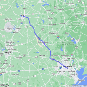
(They also provide information on how long it takes to get from point A to point B.)
Map distances, in both length and anticipated time, can be computed
with mapdist()). Moreover the function is vectorized:
mapdist(c("houston, texas", "dallas"), "waco, texas")
#  ℹ <https://maps.googleapis.com/maps/api/distancematrix/json?origins=dallas&destinations=waco,+texas&key=xxx&mode=driving>
#  ℹ <https://maps.googleapis.com/maps/api/distancematrix/json?origins=houston,+texas&destinations=waco,+texas&key=xxx&mode=driving>
#  # A tibble: 2 × 9
#    from           to               m    km miles seconds minutes hours mode
#    <chr>          <chr>        <int> <dbl> <dbl>   <int>   <dbl> <dbl> <chr>
#  1 dallas         waco, texas 151451  151.  94.1    5004    83.4  1.39 driving
# 2 houston, texas waco, texas 295091 295. 183. 10054 168. 2.79 drivingA few years ago Google has changed its API requirements, and ggmap users are now required to register with Google. From a user’s perspective, there are essentially three ramifications of this:
Users must register with Google. You can do this at https://mapsplatform.google.com. While it will require a valid credit card (sorry!), there seems to be a fair bit of free use before you incur charges, and even then the charges are modest for light use.
Users must enable the APIs they intend to use. What may appear to
ggmap users as one overarching “Google Maps” product,
Google in fact has several services that it provides as geo-related
solutions. For example, the Maps
Static API provides map images, while the Geocoding
API provides geocoding and reverse geocoding services. Apart from
the relevant Terms of Service, generally ggmap users
don’t need to think about the different services. For example, you just
need to remember that get_googlemap() gets maps,
geocode() geocodes (with Google, DSK is done), etc., and
ggmap handles the queries for you. However,
you do need to enable the APIs before you use them. You’ll only need to
do that once, and then they’ll be ready for you to use. Enabling the
APIs just means clicking a few radio buttons on the Google Maps Platform
web interface listed above, so it’s easy.
Inside R, after loading the new version of
ggmap, you’ll need provide ggmap with
your API key, a hash value (think
string of jibberish) that authenticates you to Google’s servers. This
can be done on a temporary basis with
register_google(key = "[your key]") or permanently using
register_google(key = "[your key]", write = TRUE) (note:
this will overwrite your ~/.Renviron file by
replacing/adding the relevant line). If you use the former, know that
you’ll need to re-do it every time you reset R.
Your API key is private and unique to you, so be careful not
to share it online, for example in a GitHub issue or saving it in a
shared R script file. If you share it inadvertantly, just get on
Google’s website and regenerate your key - this will retire the old one.
Keeping your key private is made a bit easier by ggmap
scrubbing the key out of queries by default, so when URLs are shown in
your console, they’ll look something like key=xxx. (Read
the details section of the register_google() documentation
for a bit more info on this point.)
The new version of ggmap is now on CRAN soon, but
you can install the latest version, including an important bug fix in
mapdist(), here with:
if(!requireNamespace("devtools")) install.packages("devtools")
devtools::install_github("dkahle/ggmap")From CRAN: install.packages("ggmap")
From Github:
if (!requireNamespace("remotes")) install.packages("remotes")
remotes::install_github("dkahle/ggmap")