![]()
![]()
Accumulated Local Effects (ALE) were initially developed as a
model-agnostic approach for global explanations of the results of
black-box machine learning algorithms (Apley, Daniel W., and Jingyu Zhu.
‘Visualizing the effects of predictor variables in black box supervised
learning models.’ Journal of the Royal Statistical Society Series B:
Statistical Methodology 82.4 (2020): 1059-1086 doi:10.1111/rssb.12377).
ALE has two primary advantages over other approaches like partial
dependency plots (PDP) and SHapley Additive exPlanations (SHAP): its
values are not affected by the presence of interactions among variables
in a model and its computation is relatively rapid. This package
rewrites the original code from the {ALEPlot}
package for calculating ALE data and it completely reimplements the
plotting of ALE values. It also extends the original ALE concept to add
bootstrap-based confidence intervals and ALE-based statistics that can
be used for statistical inference.
For more details, see Okoli, Chitu. 2023. “Statistical Inference Using Machine Learning and Classical Techniques Based on Accumulated Local Effects (ALE).” arXiv. https://doi.org/10.48550/arXiv.2310.09877.
The {ale} package currently presents three main
functions:
ale(): create data and plots for one-way ALE (single
variables). ALE values may be bootstrapped.ale_ixn(): create data and plots for two-way ALE
interactions. Bootstrapping of the interaction ALE values has not yet
been implemented.model_bootstrap(): bootstrap an entire model, not just
the ALE values. This function returns the bootstrapped model statistics
and coefficients as well as the bootstrapped ALE values. This is the
appropriate approach for small samples.You can obtain direct help for any of the package’s user-facing
functions with the R help() function, e.g.,
help(ale). However, the most detailed documentation is
found in the website
for the most recent development version. There you can find
several articles. We particularly recommend:
You can obtain the official releases from CRAN:
install.packages('ale')The CRAN releases are extensively tested and should have relatively
few bugs. However, note that this package is still in beta stage. For
the {ale} package, that means that there will occasionally
be new features with changes in the function interface that might break
the functionality of earlier versions. Please excuse us for this as we
move towards a stable version that flexibly meets the needs of the
broadest user base.
To get the most recent features, you can install the development version of ale from GitHub with:
# install.packages('pak')
pak::pak('tripartio/ale')
The development version in the main branch of GitHub is always thoroughly checked. However, the documentation might not be fully up-to-date with the functionality.
There is one more optional but recommended setup option. To enable progress bars to see how long procedures will take, you should run the following code at the beginning of your R session:
# Run this in an R console; it will not work directly within an R Markdown or Quarto block
progressr::handlers(global = TRUE)
progressr::handlers('cli')
The {ale} package will normally run this automatically
for you the first time you execute a function from the package in an R
session. To see how to configure this permanently, see
help(ale).
We will give two demonstrations of how to use the package: first, a simple demonstration of ALE plots, and second, a more sophisticated demonstration suitable for statistical inference with p-values. For both demonstrations, we begin by fitting a GAM model. We assume that this is a final deployment model that needs to be fitted to the entire dataset.
library(ale)

# Sample 1000 rows from the ggplot2::diamonds dataset (for a simple example).
set.seed(0)
diamonds_sample <- ggplot2::diamonds[sample(nrow(ggplot2::diamonds), 1000), ]

# Create a GAM model with flexible curves to predict diamond price
# Smooth all numeric variables and include all other variables
# Build model on training data, not on the full dataset.
gam_diamonds <- mgcv::gam(
  price ~ s(carat) + s(depth) + s(table) + s(x) + s(y) + s(z) +
    cut + color + clarity,
  data = diamonds_sample
)For the simple demonstration, we directly create ALE data with the
ale() function and then plot the ggplot plot
objects.
# Create ALE data
ale_gam_diamonds <- ale(diamonds_sample, gam_diamonds)

# Plot the ALE data
patchwork::wrap_plots(ale_gam_diamonds$plots, ncol = 2)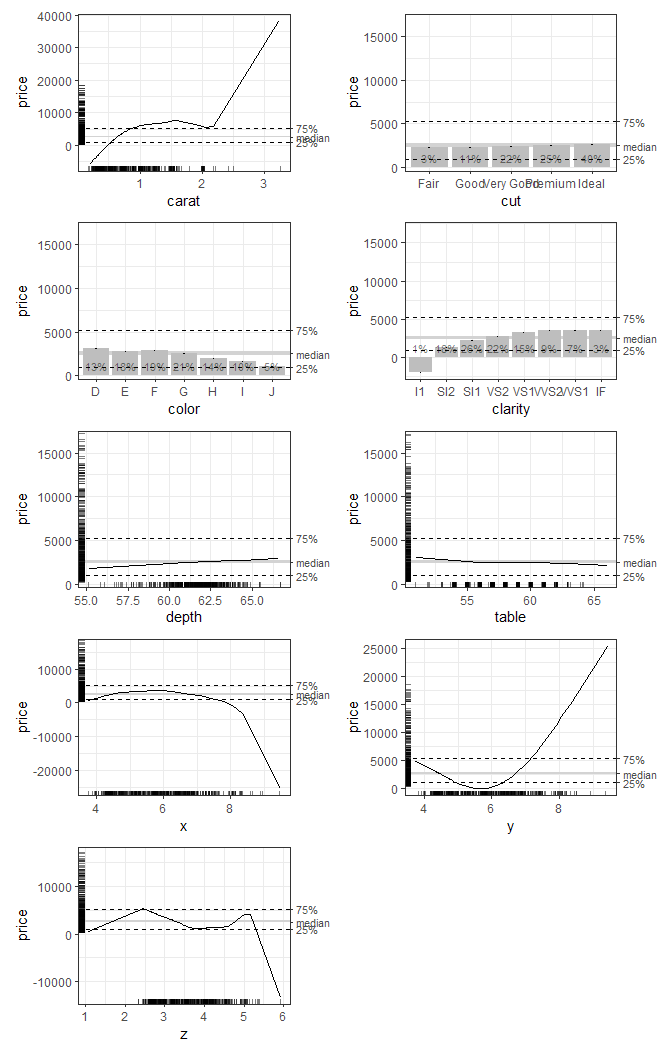
For an explanation of these basic features, see the introductory vignette.
The statistical functionality of the {ale} package is
rather slow because it typically involves 100 bootstrap iterations and
sometimes a 1,000 random simulations. Even though most functions in the
package implement parallel processing by default, such procedures still
take some time. So, this statistical demonstration gives you
downloadable objects for a rapid demonstration.
First, we need to create a p-value functions object so that the ALE statistics can be properly distinguished from random effects.
# Create p-funs object
# # To generate the code, uncomment the following lines.
# # But it is slow because it retrains the model 100 times,
# # so this vignette loads a pre-created p-values object.
# gam_diamonds_p_funs_readme <- create_p_funs(
#   diamonds_sample, gam_diamonds,
#   # Normally should be default 1000, but just 100 for quicker demo
#   rand_it = 100
#   )
# saveRDS(gam_diamonds_p_funs_readme, file.choose())
gam_diamonds_p_funs_readme <- url('https://github.com/tripartio/ale/raw/main/download/gam_diamonds_p_funs_readme.rds') |>
  readRDS()
Now we can create bootstrapped ALE data and see some of the differences in the plots of bootstrapped ALE with p-values:
# Create ALE data
# # To generate the code, uncomment the following lines.
# # But it is slow because it bootstraps the ALE data 100 times,
# # so this vignette loads a pre-created ALE object.
# ale_gam_diamonds_stats_readme <- ale(
#   diamonds_sample, gam_diamonds,
#   p_values = gam_diamonds_p_funs_readme,
#   boot_it = 100
# )
# saveRDS(ale_gam_diamonds_stats_readme, file.choose())
ale_gam_diamonds_stats_readme <- url('https://github.com/tripartio/ale/raw/main/download/ale_gam_diamonds_stats_readme.rds') |>
  readRDS()

# Plot the ALE data
patchwork::wrap_plots(ale_gam_diamonds_stats_readme$plots, ncol = 2)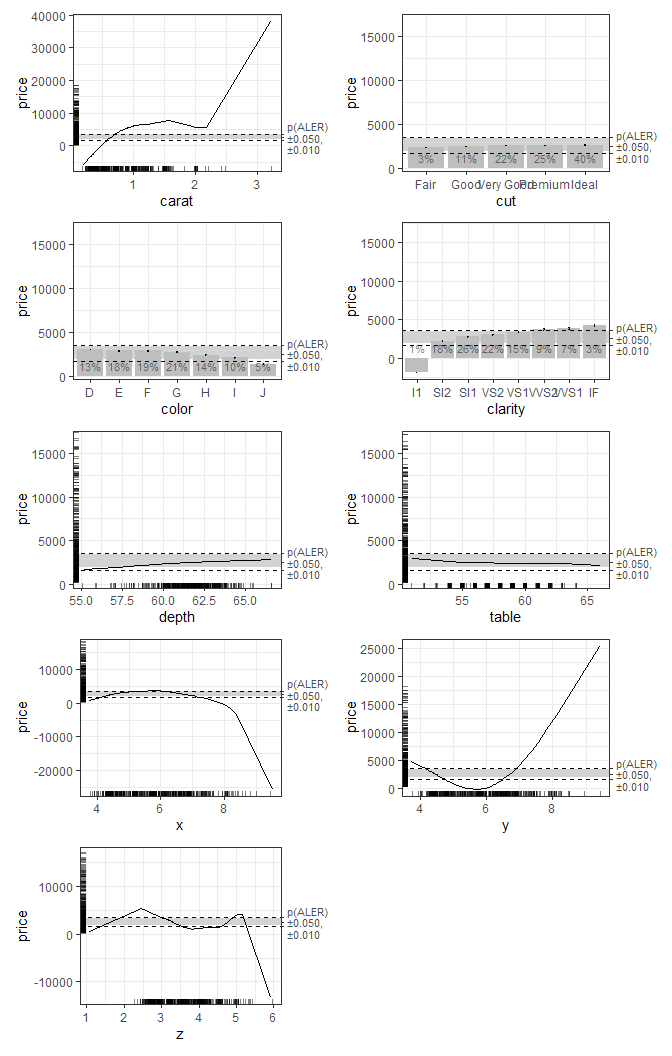
For a detailed explanation of how to interpret these plots, see the vignette on ALE-based statistics for statistical inference and effect sizes.
If you find a bug, please report it on GitHub. If you have a
question about how to use the package, you can post it on Stack Overflow with the “ale” tag.
I will follow that tag, so I will try my best to respond quickly.
However, be sure to always include a minimal reproducible example for
your usage requests. If you cannot include your own dataset in the
question, then use one of the built-in datasets to frame your help
request: var_cars or census. You may also use
ggplot2::diamonds for a larger sample.